Stormwater Engineering Fundamentals - Civil and Structural Engineer

Table of Contents

Introduction

Stormwater engineering is one of the most foundational and consequential disciplines within civil engineering. It sits at the intersection of hydrology, hydraulics, urban planning, and public safety. Yet, despite its critical importance, it is often underappreciated — until the moment a road floods, a building is inundated, or a drainage system fails during a major storm event.

Whether you are a graduate engineer stepping into your first drainage design role, a project manager overseeing infrastructure development, a council officer reviewing subdivision plans, or simply someone who wants to understand how cities manage rainfall, this article offers a thorough grounding in the fundamentals of stormwater engineering.

The content is structured to take you on a logical journey: starting from the nature of rainfall itself, through the analytical tools we use to quantify and characterise storm events, then into the methods we apply to estimate runoff, and finally through the physical infrastructure systems — inlets, pipes, and drainage networks — that manage stormwater in the real world.

What Is Rainfall?

At its most basic level, rainfall — or precipitation — is water falling from the atmosphere onto the earth’s surface. It forms the starting point of every stormwater engineering calculation. Before we can design a drain, size a pipe, or determine the appropriate freeboard for a building floor level, we need to understand how much rain is falling, how fast it is falling, and how long it will fall.

While rainfall seems conceptually simple — water falls from clouds — it is, in engineering terms, deceptively complex. Rainfall is highly variable across time, space, and intensity. It is influenced by topography, atmospheric conditions, proximity to large water bodies, seasonal patterns, and climate. In engineering practice, we must simplify this natural complexity into something we can calculate and design against. Understanding the nature of that simplification — and its limitations — is essential for competent practice.

The Hydrological Cycle

To understand rainfall, we must first understand the broader system of which it is a part: the water cycle, also called the hydrological cycle.

The water cycle describes the continuous movement of water through the earth’s surface, atmosphere, and subsurface. For stormwater engineering, the three most relevant components are:

Evaporation: Water bodies — oceans, lakes, rivers, wetlands, and soil moisture — absorb solar energy and convert liquid water into water vapour. This vapour rises into the atmosphere, carrying energy and moisture.

Condensation: As water vapour rises, it encounters cooler temperatures at higher altitudes. The vapour cools and condenses around microscopic particles (dust, pollen, sea salt) to form tiny water droplets. These droplets accumulate and aggregate to form clouds.

Precipitation: As water droplets within clouds continue to combine and grow heavier, the cloud eventually cannot support their weight. Water falls back to earth as rain, snow, sleet, or hail — depending on atmospheric conditions. In Australia and most tropical and subtropical regions, we predominantly deal with liquid rainfall.

Once rainfall reaches the earth’s surface, it follows one of three paths: it runs off over the surface into drains, streams, and water bodies; it infiltrates into the soil to replenish soil moisture and groundwater; or it is intercepted by vegetation and eventually evaporates back into the atmosphere.

Stormwater engineering is principally concerned with the first of these paths — surface runoff — though the proportion of rainfall that becomes runoff is profoundly influenced by the second and third paths.

Rainfall and Soil Infiltration

One of the most persistent misconceptions among non-engineers — and even some junior engineers — is that rainfall simply soaks into the ground. This idea leads to systematic underestimation of runoff and can result in infrastructure that is seriously undersized.

The reality is that the proportion of rainfall that infiltrates the soil depends on a complex set of interacting factors:

Rainfall intensity and duration: Light rain falling over a long period may infiltrate gradually. Heavy, intense rainfall — particularly typical of south-east Queensland and other subtropical environments — can saturate the soil rapidly or exceed its infiltration capacity, leading to surface runoff almost immediately.

Antecedent soil moisture conditions: If it has rained recently, the soil may already be saturated or near-saturated. Subsequent rainfall events will produce much higher runoff because the soil has little remaining capacity to absorb more water.

Soil composition: Sandy soils have high permeability and absorb water quickly. Clay-rich soils have much lower permeability and tend to produce greater surface runoff. The vertical layering of different soil types further complicates this.

Terrain and topography: Steep slopes accelerate surface flow and reduce the time available for water to infiltrate. Gentle slopes allow more ponding and therefore more infiltration. Converging topography concentrates overland flow and can produce rapid, intense runoff.

Land use and land cover: Natural bushland and grasslands absorb and retain more rainfall than urban developments. Roofs, roads, car parks, and other impervious surfaces shed nearly all rainfall as runoff. Agricultural cultivation and compaction can also significantly alter infiltration behaviour. The more developed and urbanised a catchment, the greater the proportion of rainfall that becomes surface runoff.

This last point has enormous implications for urban drainage design. When land is developed — when forests are cleared, soils are graded, and surfaces are paved — the hydrology of the catchment changes fundamentally. Runoff volumes increase, peak flow rates rise, and the time between rainfall onset and peak flow (known as the response time or time of concentration) decreases. Drainage infrastructure must be sized to accommodate these changes.

Groundwater and Baseflow

Even after a storm event ends and surface runoff ceases, catchments may continue contributing flow to creeks and drainage systems for hours, days, or even weeks. This sustained flow comes from groundwater, and it is referred to in hydrology as baseflow.

During and after rainfall, some water infiltrates deeply enough to recharge groundwater aquifers. This groundwater moves slowly through permeable rock and soil layers and eventually discharges into rivers, creeks, and drainage channels. In some catchments, this baseflow can be substantial and long-lasting.

The factors that govern groundwater behaviour include the characteristics of the aquifer (its porosity and permeability), the rate at which it is being recharged by infiltrating rainfall, the rate of extraction (such as for irrigation or groundwater supply), and seasonal variability. During extended dry periods, baseflow may cease entirely; during and after wet seasons, it may sustain significant flows well beyond the end of any individual storm.

For drainage engineers, baseflow is rarely a primary design consideration for urban pit-and-pipe systems. However, it is highly relevant to the design of waterway channels, detention basins, culverts, and any infrastructure that must manage sustained flows beyond the peak of a single storm event.

Simplifying Rainfall for Engineering Design

Because natural rainfall is so complex — variable in intensity, duration, spatial distribution, and frequency — engineers must adopt simplified representations that can be used reliably in design calculations. The concept of the design storm is central to this simplification.

A design storm is a hypothetical rainfall event, constructed from historical rainfall data, that represents a particular combination of intensity, duration, and frequency. Rather than attempting to predict exactly when or how intensely it will rain, engineers ask: “What is the worst storm of a given rarity that I should design for?” The design storm provides a standardised answer to that question.

Design storms are characterised by two key parameters:

Storm burst duration: The length of time over which peak rainfall intensity is sustained.
Storm frequency: How often, statistically, we would expect a storm of that intensity and duration to occur.

A common example would be designing a stormwater pipe for the “10% AEP event with a 10-minute storm burst duration” — meaning the pipe should be capable of handling the intensity of rainfall that has a 10% chance of being equalled or exceeded in any given year, sustained for 10 minutes.

In Australian practice, drainage infrastructure is typically classified as either minor or major systems, each designed to a different storm frequency:

Minor systems (piped underground networks, kerb-and-channel flows) are typically designed for more frequent events — ranging from 63% AEP to 10% AEP depending on the land use category.
Major systems (overland flow paths, roads used as drainage corridors, drainage reserves) are typically designed for rarer, more extreme events, commonly the 1% AEP (1-in-100-year) event.

This two-system approach acknowledges that no practical pipe network can be designed to carry all stormwater underground in an extreme storm. Instead, the philosophy is that the minor system handles frequent events efficiently while the major system provides a safe pathway for rarer, larger events — with flow routed along roads, parks, and dedicated drainage reserves rather than flooding buildings.

Anatomy of a Storm

The Phases of a Rainfall Event

To design drainage infrastructure properly, engineers need to understand not just the total volume of rain that falls, but how that rain is distributed through time. A rainfall event is not uniform — it has a structure, a rising limb, a peak, and a falling limb. Understanding this structure is essential for correctly applying design tools like the Rational Method.

A complete rainfall event can be divided into four phases:

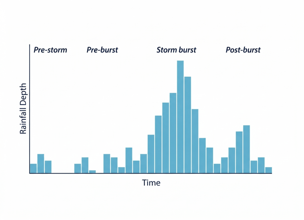
Pre-storm rainfall: This is low-level, often intermittent rainfall that precedes the main storm event. It may occur hours before the storm proper begins. Its significance lies in its effect on soil moisture: pre-storm rainfall begins to saturate catchments, reducing their capacity to absorb subsequent rainfall and increasing the proportion that becomes runoff.

Pre-burst rainfall: This phase immediately precedes the storm burst. The storm is still developing, and rainfall intensity is increasing but has not yet reached its peak. Pre-burst rainfall continues to wet up the catchment and contributes to the antecedent moisture conditions that influence the runoff coefficient applied in design calculations.

Storm burst: This is the critical phase — the peak of the storm event when rainfall intensity is at its maximum. The storm burst is characterised by the highest rainfall rates, the greatest volumes per unit time, and consequently the greatest potential for producing damaging surface runoff. It is this phase that engineers focus on when designing stormwater infrastructure, because it is during the storm burst that flows peak and systems are tested most severely.

Post-burst rainfall: After the peak intensity, rainfall gradually diminishes. The post-burst phase is important for understanding the total volume of water entering drainage systems and for assessing whether detention or retention facilities can safely drain before the next event, but it is less critical than the storm burst for sizing pipes and inlets.

In engineering practice — particularly when applying the Rational Method — we focus on the storm burst. The Rational Method is designed to estimate the peak discharge rate, which occurs during the storm burst when rainfall intensity and the drainage catchment are both contributing maximally to flow.

Storm Frequency

How We Classify Storm Rarity

One of the most important concepts in stormwater engineering is storm frequency — the statistical characterisation of how rare a given storm event is. This is the foundation for making rational decisions about what level of protection to provide, what size of pipe to install, and what floor levels to set for buildings.

Storms are broadly grouped into frequency categories:

Very frequent (high AEP values)
Frequent
Infrequent
Rare
Extremely rare
Extreme (including the Probable Maximum Precipitation)

Each category corresponds to specific numerical values that allow rigorous engineering calculation.

The Three Ways to Express Storm Frequency

Storm frequency is expressed in three related but distinct ways:

Exceedances per Year (EY): This expresses how many times per year, on average, a storm of a given intensity might be equalled or exceeded at a particular location. For example, a storm that occurs six times per year on average has an EY value of 6. This metric is particularly useful for very frequent events.

Annual Exceedance Probability (AEP): This is the probability that a storm of a given magnitude will be equalled or exceeded in any given year, expressed as a percentage. A 50% AEP storm has a 50% chance of being equalled or exceeded in any one year. A 1% AEP storm has a 1% chance. AEP is now the preferred terminology in Australian engineering practice.

Average Recurrence Interval (ARI): This is the average number of years between occurrences of a storm of a given magnitude. It is mathematically related to AEP: a 1% AEP storm corresponds to a 100-year ARI (often called the “1-in-100-year storm”). While the ARI terminology is still understood and widely used colloquially, current Australian practice favours AEP because it avoids the common misunderstanding that a “100-year storm” can only happen once per century.

The relationship between these measures is straightforward: an AEP of 1% means an ARI of 100 years; an AEP of 10% means an ARI of 10 years; an AEP of 63.2% means an ARI of approximately 1 year (the annual storm). Understanding this equivalence is essential for interpreting design standards, client briefs, and council requirements.

Why Frequency Matters for Design

Different types of infrastructure are designed to different storm frequencies, reflecting differences in consequence, cost, and acceptable risk:

Stormwater quality (water sensitive urban design) measures are commonly designed for very frequent events (63% AEP or greater), because pollutant loads are dominated by frequent small storms.
Minor drainage systems (kerb and channel, pit-and-pipe) are designed for events ranging from 63% AEP to 10% AEP, depending on the land use category and the road type.
Roofwater drainage and eaves gutters are typically designed for the 10% AEP (10-year ARI) event.
Major drainage systems and floodplain management are typically assessed against the 1% AEP (100-year) event.
Residential building floor levels are set with reference to the 1% AEP flood level.
Critical infrastructure (hospitals, emergency services, evacuation routes) must be assessed against rarer events — 0.2% AEP (500 years) or 0.5% AEP (200 years).

These frequency requirements are codified in local government planning schemes, state-based standards (such as the Queensland Urban Drainage Manual, QUDM), and national references (such as Australian Rainfall and Runoff, AR&R). Engineers must understand both the numerical requirements and the engineering rationale behind them.

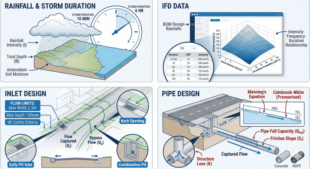
Intensity-Frequency-Duration (IFD) Data

The IFD Framework

One of the most important tools in an Australian stormwater engineer’s toolkit is the Intensity-Frequency-Duration (IFD) relationship — a data framework that quantifies the expected rainfall intensity for any combination of storm duration and Annual Exceedance Probability at a given location.

The three axes of IFD data are:

Intensity (I): The rate at which rain falls, measured in millimetres per hour (mm/h). Higher intensity means more rain per unit of time. Rainfall intensity can also be expressed as a depth in millimetres (mm) when multiplied by the storm duration.
Frequency: The probability of the storm occurring in any given year, expressed as an AEP (%). Rarer storms (lower AEP) are associated with higher intensities.
Duration: The length of time over which the storm burst is sustained, measured in minutes or hours. Shorter storms tend to be more intense; longer storms have lower average intensities but deliver greater total depths.

The IFD relationship at any location is derived from decades of historical rainfall records. In Australia, the Bureau of Meteorology (BOM) maintains and publishes IFD data for every location in the country via its Design Rainfalls website (bom.gov.au/water/designRainfalls/revised-ifd). Engineers access these tables by entering the geographic coordinates of their project site and receive tabulated rainfall intensities for a range of durations (from 1 minute to 72 hours or more) and AEP values (from 63.2% down to 1% and beyond).

Reading an IFD Table

IFD data is typically presented as a table, with storm durations in the rows and AEP values in the columns. Each cell in the table contains a rainfall intensity value in mm/h.

For example, a typical IFD table for a site in Sydney, NSW might show:

At 10-minute duration and 1% AEP: 250 mm/h
At 10-minute duration and 10% AEP: 172 mm/h
At 30-minute duration and 1% AEP: 151 mm/h
At 30-minute duration and 10% AEP: 101 mm/h

Two important trends are immediately apparent from any IFD table:

As storm frequency decreases (lower AEP), intensity increases. This makes physical sense — rarer storms are associated with more extreme rainfall rates. A 1% AEP storm is considerably more intense than a 10% AEP storm of the same duration.

As storm duration increases, intensity decreases. This also makes physical sense — while it is possible to sustain very high rainfall rates for a few minutes, it is not physically sustainable for hours. Longer-duration averages are therefore lower than short-duration peaks.

These two trends are fundamental to how engineers select design parameters. The “critical storm duration” for a given catchment — which produces the maximum peak flow — depends on the catchment’s response time (time of concentration) and must be carefully determined, not arbitrarily assumed.

IFD and Local Variability

IFD data varies enormously by location. A site in coastal Queensland will have much higher rainfall intensities than a site in arid Western Australia. Even within a single city, there can be significant variation due to local topography, proximity to the coast, and orographic effects (rainfall enhancement by hills and ridges).

This is why engineers must always obtain site-specific IFD data from BOM rather than applying generic values. Using incorrect IFD data — even data from a nearby location — can lead to systematic under- or over-design with serious consequences.

The revised IFD data published by BOM incorporates far more comprehensive historical records and statistical methods than earlier versions. Engineers should always use the most current available data and be alert to updates that may affect ongoing projects.

The Rational Method

Overview

Once we understand the nature of rainfall and can quantify design storm parameters, the next challenge is estimating how much surface runoff will be generated from a catchment and at what peak flow rate. This is the domain of hydrological analysis.

For small to medium urban catchments — which constitute the vast majority of stormwater drainage design problems in civil engineering practice — the Rational Method is the standard tool. It has been used by engineers for over 150 years and, despite its simplicity, remains widely applicable and broadly accepted when used with care and understanding.

The Rational Method is expressed by a deceptively simple formula:

Q = CIA / 360

Where:

Q = Peak flow rate (m³/s)
C = Coefficient of runoff (dimensionless)
I = Rainfall intensity (mm/h) for the design storm duration equal to the time of concentration
A = Catchment area (ha)
360 = A unit conversion factor

The Assumptions Behind the Rational Method

The Rational Method is not a universal tool — it is an approximation that relies on two key assumptions:

The storm burst duration equals the time of concentration of the catchment. This condition produces the maximum peak discharge because it ensures that the entire catchment is contributing runoff to the outlet simultaneously when rainfall intensity is at its peak.
The entire catchment receives uniform rainfall throughout the storm burst. This is a simplification — real storms are not spatially uniform — but it is reasonable for small catchments where the spatial variability of rainfall intensity is not dominant.

For large catchments, complex catchments with multiple sub-areas and flow paths, or situations where temporal storage effects are important, more sophisticated hydrological models may be required. The Rational Method is appropriate for catchments up to a few hundred hectares in typical urban drainage applications, but engineers must exercise judgement about its limitations on larger or more complex catchments.

Time of Concentration

The time of concentration (tc) is one of the most important — and often most carefully estimated — parameters in the Rational Method. It is defined as the time required for stormwater runoff to travel from the hydraulically most remote point of the catchment to the outlet.

The critical word in that definition is time, not distance. The “most remote point” is the point that takes the longest to drain, which is not necessarily the geographically most distant point. A point at the top of a long, flat, grassy slope may have a longer time of concentration than a point at a similar distance down a steep paved surface, because water moves more slowly across the former.

Time of concentration is the sum of the travel times along all components of the flow path from the catchment divide to the outlet. Depending on the nature of the catchment, this flow path may include some or all of the following components:

Roof to Main System Connection

In urban catchments with connected roof drainage, stormwater falls on a roof, flows via gutters and downpipes into a subsoil or surface connection, and enters the street drainage system. The travel time for this component is relatively short — typically a few minutes — but must be accounted for in the time of concentration calculation for small lot-level catchments.

Kerb Flow

Water that reaches the road surface flows along the kerb and channel toward the nearest stormwater inlet. This is a surface flow component characterised by the road’s longitudinal grade and crossfall. Kerb flow velocity is generally moderate, and travel times depend on the distance from the hydraulically remote point to the inlet.

Pipe Flow

Where stormwater has already entered an underground pipe system, it travels through the pipe network. Pipe flow velocities are typically higher than surface flow velocities (often 1.5–4 m/s or more), so the travel time contribution from pipe flow components is relatively short per unit distance.

Channel Flow

In rural or semi-rural settings, stormwater may flow through engineered channels — table drains, swales, or lined stormwater channels. Channel flow velocities depend on the channel geometry, slope, and roughness, and travel times can be significant for longer flow paths.

Overland Sheet Flow

Sheet flow is the thin, uniform layer of water that moves across a surface before concentrating into defined flow paths. It occurs at the very beginning of the flow path, typically across the ground surface from the catchment divide before reaching any concentrated flow path. Sheet flow velocities are very low — typically only a few centimetres per second — and therefore contribute disproportionately to the time of concentration.

Importantly, sheet flow rarely persists for more than about 50 metres before concentrating into a rill, runnel, or defined flow path. Engineers applying the Kinematic Wave Equation or other sheet flow formulae should be careful not to apply them over distances greater than this without justification.

Concentrated Overland Flow

Once sheet flow has concentrated, it becomes concentrated overland flow, moving through shallow natural channels or depressions across the surface. This is the transition between sheet flow and defined channel flow. Travel times for concentrated overland flow are faster than for sheet flow but slower than for defined channel flow.

Understanding the composition of the flow path — which components are present, in what proportions, and with what characteristics — is fundamental to correctly calculating the time of concentration and therefore correctly applying the Rational Method.

The Runoff Coefficient (C)

The runoff coefficient C is the parameter in the Rational Method that accounts for the proportion of rainfall that actually becomes surface runoff. It is a dimensionless number between 0 and 1, where:

C = 0 means no rainfall becomes runoff (completely pervious surface)
C = 1 means all rainfall becomes runoff (completely impervious surface)

In practice, C values range from around 0.1–0.2 for natural bushland or large-lot rural residential areas, to 0.9–0.95 for highly impervious urban surfaces such as car parks or commercial precincts.

The runoff coefficient accounts not just for impervious cover but also for infiltration losses, depression storage (small depressions that trap water before it can run off), and interception by vegetation. It is a lumped parameter that incorporates several physical processes into a single number — which is both its strength (simplicity) and its weakness (imprecision).

In Australian practice, QUDM provides tables of recommended C values for different land use categories and surface types. Engineers select appropriate C values based on the proportion of impervious area within the catchment and the type of land use.

For mixed catchments containing both impervious and pervious surfaces, a composite C value is calculated as the area-weighted average of the individual C values for each surface type.

It is also important to note that C values in the Rational Method are frequency-dependent (denoted Cy). Rarer storms, which tend to produce higher soil saturation, are associated with slightly higher runoff coefficients. QUDM provides frequency adjustment factors to account for this.

Rainfall Intensity in the Rational Method

With the time of concentration determined and the design storm frequency selected, the engineer retrieves the corresponding rainfall intensity from the IFD table for the project location. This intensity (I), combined with C and A, gives the peak discharge Q.

It is worth noting that the relationship between storm duration and peak discharge is not monotonic. For a given catchment:

Very short storm durations produce high rainfall intensity but don’t last long enough for the whole catchment to contribute.
Very long storm durations produce low intensity but allow the whole catchment to contribute.

The maximum peak discharge occurs when the storm duration equals the time of concentration — which is precisely the assumption embedded in the Rational Method. This is why correctly calculating tc is so critical.

Catchment Area (A)

The catchment area (A) is the plan area of land that drains to the point of interest for which peak discharge is being calculated. It is measured in hectares (ha) in the Rational Method formula as presented above.

Catchment boundaries are determined by the topography — specifically, by the ridgelines and high points that form the watershed divide. Water falling on one side of a watershed divide will drain to one outlet; water falling on the other side drains elsewhere.

In practice, catchment boundaries are delineated using contour maps, survey data, aerial imagery with terrain analysis, and — increasingly — LiDAR (Light Detection and Ranging) digital terrain models. For urban catchments, the delineation is complicated by the presence of kerbs, inlets, pipes, and other drainage infrastructure that redirects natural drainage patterns. Engineers must carefully trace how stormwater actually moves through the urban fabric, not simply how the natural terrain would suggest it moves.

The outlet point — the point at which peak discharge is being calculated — can be any location: a proposed inlet, the low point of a sag, a property boundary, the end of a drainage channel, or the entry to a detention basin. For complex catchments with multiple sub-catchments, peak discharge is typically calculated at multiple points along the drainage system.

Peak Discharge (Q)

The output of the Rational Method is the peak discharge Q — the maximum rate of stormwater runoff expected at the design point for the design storm. It is expressed in cubic metres per second (m³/s).

Peak discharge is the fundamental currency of stormwater drainage design. Once you know Q, you can:

Size stormwater pipes to carry that flow without surcharging
Design stormwater inlets to capture that flow within acceptable flow width limits
Size drainage channels to convey that flow at safe velocities and depths
Design detention basins to attenuate that flow to an acceptable pre-development level
Assess the flooded width and depth on roads, and determine whether it meets safety criteria
Set floor levels for buildings to ensure they are above the design flood level plus required freeboard

The Rational Method, for all its simplicity, is a powerful tool when applied with a thorough understanding of its assumptions, inputs, and limitations.

Inlet Design

The Urban Drainage Context

In urban environments, stormwater must be managed within tight spatial constraints. Roads are busy with vehicles and pedestrians. Properties are densely developed. There is little space for broad, shallow overland flow paths. The challenge of urban stormwater management is to intercept surface runoff quickly and efficiently and convey it underground through a pipe network to a suitable point of discharge.

This is the purpose of the longitudinal drainage system — the familiar network of inlets, pits, and underground pipes that forms the backbone of urban stormwater management. The system is called “longitudinal” because it runs along the road corridor, intercepting kerb flow and directing it underground.

The design of this system involves close integration between road geometry and stormwater hydraulics. The geometry of the road — its longitudinal grade, crossfall, width, and kerb type — directly determines how stormwater flows and accumulates on the road surface. The drainage infrastructure — inlets, pipes, and outlets — must be designed to manage that flow safely and within regulatory limits.

A key insight for engineers working in this field is that road design is stormwater design. Every decision about road geometry has hydraulic consequences. Conversely, every stormwater calculation feeds back into constraints on road geometry: how wide can a road be before flows become unsafe? How flat can a grade be before ponding in sags becomes excessive? How much of the road surface can we allow to flood before pedestrian or vehicle safety is compromised?

Types of Stormwater Inlets

Stormwater inlets are the structures that capture surface runoff from roads, footpaths, and other paved surfaces and direct it into the underground pipe network. Two broad classifications apply:

Sag inlets are located at the low point (sag) of the road profile, where water naturally pools. All water flowing toward the sag must eventually pass through the inlet — there is no bypass. This makes sag inlets critical safety points: if a sag inlet is blocked or undersized, water will pond indefinitely, potentially to significant depths.

On-grade inlets are located on a sloping road section where water flows longitudinally along the road before reaching the inlet. Some water is captured by the inlet; the remainder bypasses it and continues downstream. On-grade inlets are designed to achieve a target capture efficiency — typically not 100%, as some bypass to the next downstream inlet is expected and planned for.

Physically, stormwater inlets take several forms:

Kerb inlets (side entry pits): These capture water through an opening in the kerb face. The opening, called the kerb opening or lintel, is typically 0.9 m to 1.5 m long. Behind the lintel is a trough that deflects flow downward into the underground chamber. Kerb inlets are the most common type in Australian urban environments.

Grated inlets: These capture water through a grate set flush with the road or footpath surface. They are effective at capturing sheet flow as well as kerb flow, but are vulnerable to blockage from leaves, grass clippings, and other debris — and can pose a hazard to cyclists if grate bars are oriented parallel to the direction of travel.

Combination inlets (gully pits): These combine both a kerb opening and a grate, offering greater capture efficiency and providing redundancy if one component is partially blocked.

Field inlets (drop inlets): These are grated pits set into grassed or landscaped areas to collect concentrated overland flow or shallow sheet flow from parks, sports fields, and other open areas. They may be flush-mounted (grate level with the ground surface), elevated on an apron, or fitted with a dome screen to reduce debris ingress.

All inlets require regular maintenance to ensure they remain operational. Blockage by leaves, grass clippings, soil, and other debris is one of the most common causes of localised flooding. Engineers designing drainage systems should consider maintenance access and debris management as integral parts of the design.

Flow Limits: The Safety Framework

Before calculating how much flow a given inlet will capture, engineers must first ensure that the approach flow — the flow heading toward the inlet — falls within acceptable safety limits. These limits exist for two fundamental reasons: vehicle safety and pedestrian safety.

Water flowing over road surfaces creates hazards. Shallow, fast-moving water can cause vehicles to hydroplane and lose steering control. Deeper water can cause vehicles to stall or be swept off the road. Pedestrians may lose their footing in fast-moving shallow water, and children in particular can be overwhelmed by depths that an adult might consider inconsequential.

Australian standards — codified in QUDM and adopted by most state and local governments — define limits for:

Flow width: The lateral spread of stormwater across the road surface. For minor storms on major roads, flow width is typically limited to the parking lane width (approximately 2.5 m), ensuring that at least one traffic lane remains clear. On minor roads, flow may be allowed to extend to the full pavement width with zero depth at the crown under certain conditions. At pedestrian crossings and bus stops, flow width is limited to just 0.45 m, reflecting the vulnerability of pedestrians in these locations.

Flow depth: The depth of water at the kerb. Limits vary depending on whether flow is longitudinal (along the road) or transverse (crossing the road) and whether the situation poses a risk to life. A common limit for minor storms at road sags (still water conditions) is 300 mm maximum depth.

Depth-velocity product (dV): This is the product of water depth and flow velocity, measured in m²/s. It is the most sophisticated of the safety metrics and accounts for the fact that fast-moving shallow water can be as dangerous as slow-moving deep water. Limits typically range from 0.3 m²/s for situations with risk to life (such as causeways with transverse flow) to 0.6 m²/s for longitudinal flow on major roads with lower risk.

These limits apply differently to minor and major storm events and vary with the consequence of exceedance. Engineers designing drainage infrastructure must check all relevant flow limits for both minor and major design storms before proceeding with inlet sizing.

Flow Terminology: Qc, Qa, Qi, Qb

A consistent and precise vocabulary is essential for drainage design. The following four flow terms are fundamental:

Qc — Catchment flow: The flow generated by the local catchment that drains directly to a particular inlet. Calculated using the Rational Method for the local catchment contributing to that pit.

Qa — Approach flow: The total flow arriving at an inlet from upstream. For the first inlet in a system (at the top of the catchment), Qa = Qc. For downstream inlets, Qa = Qc (local catchment) + Qb from upstream (bypass flow from the upstream inlet that was not captured).

Qi — Inflow: The flow actually captured by the inlet and conveyed underground through the pipe network. Qi depends on the hydraulic efficiency of the inlet, which is determined from inlet capture charts.

Qb — Bypass flow: The flow that is not captured by the inlet and continues past it as surface flow, potentially reaching the next downstream inlet. Qb = Qa − Qi.

This framework reflects the reality that no inlet captures 100% of its approach flow (except at sag conditions with sufficient ponding depth). Designing a drainage system requires tracking the bypass flow from each inlet and adding it to the catchment flow at the next downstream inlet to determine the approach flow at that location.

Understanding how catchments are divided, how flow accumulates through a system, and how bypass propagates downstream requires a thorough grasp of the local topography — where road crests split flow in opposing directions, where lots drain to the road, where kerb returns redirect flow at intersections, and where sag points force all flow through a single inlet.

Inlet Capture Charts

The hydraulic performance of a stormwater inlet — how much flow it captures under various conditions — cannot be determined by inspection alone. It requires either mathematical hydraulic analysis or laboratory testing, and the results are typically presented in inlet capture charts.

Inlet capture charts are graphical or tabular representations of an inlet’s hydraulic behaviour under different approach flow and road geometry conditions. They are derived from analytical equations (based on weir and orifice flow theory) or from physical hydraulic laboratory testing, and they allow engineers to predict the capture efficiency of a specific inlet type under specific road geometry conditions.

For sag inlets, hydraulic performance is governed primarily by the depth of ponding above the inlet opening. The inlet behaves as a weir (when water depth is shallow relative to the opening height) or as an orifice (when water depth is great relative to the opening). As ponding depth increases, capture capacity increases — but so does the risk of exceeding flow depth safety limits.

For on-grade inlets, hydraulic performance is governed by the road’s longitudinal grade, crossfall, and the inlet’s physical dimensions. Higher grades produce faster flow with narrower spread and shallower depth, which reduces capture efficiency. Lower grades produce slower, wider, deeper flow, which improves capture efficiency. Engineers use capture charts to determine the combination of inlet type, size, and spacing that achieves the desired level of performance within the road geometry and flow limit constraints.

Piped Network Hydraulics

Elements of a Piped Drainage System

Once stormwater is captured by an inlet, it enters an underground piped network. This network consists of four main elements:

Drainage inlets: Described in the previous section — the interface between the surface and underground systems.

Access chambers: Structures that provide physical access to the underground pipe network for inspection, maintenance, cleaning, and asset management. Access chambers are placed at changes in pipe direction, grade, and size; at junctions where tributary pipes connect to the main line; and at regular intervals along straight pipe runs to ensure the entire system can be accessed. Without adequate access chambers, maintaining a drainage system is practically impossible.

Underground pipes: Circular or elliptical conduits (most commonly reinforced concrete or high-density polyethylene) that convey captured stormwater from inlets toward the point of discharge. Pipes are sized to convey the design flow at acceptable velocities — fast enough to maintain self-cleansing (typically above 0.9 m/s) but not so fast as to cause scouring or structural damage. Minimum pipe diameters for public drainage systems are typically 375 mm or 450 mm to allow for reasonable access and self-cleansing.

Outlets: The point at which the piped network discharges into a receiving water body, detention basin, bioretention system, or another drainage system. Outlets are typically fitted with a headwall — a concrete or masonry structure that provides a stable, controlled point of discharge, protects the pipe end from erosion, and manages the hydraulic transition from pipe flow to open channel flow. Outlet design must also consider scour protection at the point of discharge to prevent erosion of the receiving land or water body.

Key Pipe Terminology

Precise vocabulary is essential in piped drainage design. The following terms are fundamental:

Invert: The lowest internal point of a pipe cross-section — the floor of the pipe at any given location. Invert levels are the primary reference for pipe alignment and grade.

Obvert: The highest internal point of a pipe cross-section — the ceiling of the pipe.

Crown: The highest external point of the pipe — the top of the pipe including the pipe wall thickness.

Pipe slope (So): The grade of the pipe, expressed as a ratio (e.g., 1:200 = 0.005 m/m). This is the physical slope of the pipe barrel and is not the same as the friction slope used in hydraulic calculations.

Cover: The vertical distance from the finished surface level to the crown of the pipe. Minimum cover requirements protect pipes from damage by vehicles and ensure structural integrity.

Pit drop: The difference in invert level between the inlet pipe(s) and the outlet pipe at a pit structure. A pit drop is typically provided to account for energy losses at the junction and to maintain hydraulic grades. Without adequate pit drops, the hydraulic grade line may rise above expected levels and cause surcharging.

Pipe length: For design purposes, pipe length is measured between the centres of the upstream and downstream pit structures — not between the end faces of the pipe. This convention accounts for the fact that head losses occur within the pit structure itself.

Pressure Head and Hydraulic Grade Line

Understanding how water moves through a pipe network requires an understanding of pressure head and the Hydraulic Grade Line (HGL).

Pressure head is the force that water exerts due to the weight of water above it. It is measured in metres of water. In a pipe system, pressure head at any point drives the flow of water through the pipe — higher pressure at one end and lower pressure at the other creates a pressure gradient that moves water from high to low.

The velocity of flow through a pipe is directly related to the pressure gradient. Greater pressure head differences (steeper hydraulic gradients) produce faster flow. This is why the hydraulic grade line — not the physical pipe slope — is the governing factor in determining flow velocities.

The Hydraulic Grade Line (HGL) is a conceptual line drawn through a pipe network that represents the pressure head at every point. Physically, the HGL represents the level to which water would rise in a vertical standpipe inserted into the pipe at that point. Key characteristics:

When the HGL is below the pipe crown (obvert), the pipe is flowing partially full — open channel conditions prevail.
When the HGL is at the pipe obvert, the pipe is flowing full but not under pressure — the boundary condition between open channel and pressure flow.
When the HGL is above the pipe obvert, the pipe is flowing under pressure — pressurised flow conditions.

For each pipe reach, the HGL drops along the pipe due to friction losses — energy dissipated by the friction between the flowing water and the pipe wall. This head loss is calculated using the equation:

hf = Sf × L

Where hf is the friction head loss, Sf is the friction slope, and L is the pipe length. Note that the friction slope Sf is not the same as the pipe slope So — they are related by the flow conditions and pipe properties.

At each junction, bend, change in pipe size, or other discontinuity, additional energy losses occur due to the disruption of the flow pattern. These are called structure losses (or minor losses), calculated as:

hs = K × (Vo² / 2g)

Where hs is the structure head loss, K is a dimensionless structure loss coefficient (which varies depending on the type of junction and the flow conditions), Vo is the downstream pipe velocity, and g is gravitational acceleration (9.81 m/s²).

Total Energy Line

The Total Energy Line (TEL) sits above the HGL by a distance equal to the velocity head (Vo²/2g). While the HGL represents pressure energy, the TEL represents the total energy available — pressure energy plus kinetic energy. Flow in any pipe system moves from high total energy to low total energy; it is the TEL, not the HGL, that correctly represents the driving head for flow.

In most practical drainage design, the HGL is the primary working tool, and the TEL is referenced when precision is required or when velocity heads are significant (as in high-velocity systems). In still-water conditions — such as within a detention basin — the HGL and TEL coincide.

Water Surface Elevation in Pits

The actual water level within a pit structure (the water surface elevation, or WSE) is typically somewhat higher than the theoretical HGL at that point. This is because the inflow of water into the pit and the redirection of flow into the outlet pipe create additional turbulence and energy dissipation that the theoretical HGL does not fully capture.

Separate structure loss coefficients (Kw) are used to compute the WSE within a pit, distinct from the Ku coefficient used for HGL calculations. The WSE is the critical level for checking that water does not surcharge out of the pit grate during a design event, and a minimum freeboard of 150 mm is required between the calculated WSE and the pit lid or grate level.

Hydraulic Models for Pipe Design

Three levels of hydraulic modelling are used for piped drainage systems:

Simple, steady flow, open channel model: This is the most straightforward approach. It assumes the HGL sits at the pipe obvert throughout the system (pipes flowing full but not under pressure). Manning’s Equation is used to calculate the capacity of each pipe, and pipes are sized so that their full-flow capacity equals or exceeds the design discharge. This method is conservative and practical for initial design and checking, but it does not account for the actual distribution of pressure through the system or the energy losses at pit structures.

Manning’s Equation:
V = (1/n) × R^(2/3) × S^(1/2)

Combined with the volumetric flow rate equation Q = VA, this gives the pipe carrying capacity for any combination of pipe size, roughness, and slope.

Steady flow, pressurised grade line model: This more sophisticated approach explicitly calculates the HGL through the system, accounting for friction losses in pipes and structure losses at pits. It recognises that the HGL may be above the pipe obvert (pressurised conditions) or below it (open channel conditions) and traces the hydraulic grade throughout the system. This is the appropriate model for detailed design, as it correctly determines whether the HGL remains below pit grate levels and whether freeboard requirements are satisfied. The Colebrook-White equation is used for friction losses in pressurised conditions.

Complex, unsteady flow model: This advanced approach uses numerical modelling software to simulate the time-varying behaviour of the drainage system throughout the entire design storm event. Water levels fluctuate as the storm rises and falls, and the model captures the dynamic interaction between inflows, storage, and outflows. This approach is used when detailed assessment of volume storage, detention behaviour, or complex system interactions is required. It requires significantly more data and expertise to apply correctly.

In practice, the open channel model is appropriate for initial concept design and quick checks. The pressurised grade line model is required for detailed design submissions. Unsteady flow modelling is used for major drainage studies, detention basin design, and situations where the simplified assumptions of the first two models are insufficient.

Tailwater Conditions and Starting HGL

One of the most consequential decisions in piped drainage design is the selection of the starting HGL — the water level at the downstream end of the system, from which the hydraulic analysis propagates upstream. This is called the tailwater condition.

The tailwater is the water level in the receiving body at the point where the drainage system discharges. It may be the level in a creek, canal, detention basin, ocean outfall, or another drainage system. The tailwater condition sets the boundary condition for the entire upstream hydraulic analysis.

The rules for establishing the starting HGL are:

If the tailwater level (TWL) is above the pipe obvert level (OL): The HGL is set to the tailwater level (HGL = TWL). The pipe outlet is submerged.
If the TWL is below the obvert level but above the critical depth (dc) of flow in the pipe: The HGL is set to the pipe obvert level (HGL = OL). This represents the transition between free discharge and submerged outlet conditions.
If the TWL is below the pipe invert level, or below the critical depth: The HGL is set to the normal flow depth in the pipe (HGL = dn). Free outlet conditions prevail.

Critical depth is the depth at which specific energy is minimised for a given discharge — a fundamental concept in open channel hydraulics. For circular pipes, critical depth is typically around 80–90% of the pipe diameter for full-flow conditions.

The choice of tailwater condition has significant implications for the hydraulic performance of the upstream system. A high tailwater raises the HGL throughout the system, potentially causing surcharging. A low tailwater allows the system to drain more freely and operates with lower HGL levels.

In urban drainage design, the tailwater level is often a function of the performance of the downstream drainage system — which may or may not have been analysed. Engineers must liaise with the relevant authority to agree on an appropriate tailwater assumption, particularly when connecting new systems to existing infrastructure.

Connecting to Existing Pipe Networks

One of the most challenging situations in drainage design is connecting a new development’s drainage system to an existing downstream network. This scenario raises fundamental questions about the capacity of the existing system to accept additional flow.

Urbanisation and densification systematically increase stormwater discharge from catchments. When land is developed, impervious cover increases, C values rise, and peak discharges grow. If this increased discharge is fed into an existing system that was designed for the original (lower) level of development, the existing system may be overwhelmed.

This is not a hypothetical concern — it is a common and recurring problem in developing cities. Systems that were designed to handle the flows from a semi-rural catchment may be seriously undersized once that catchment is fully urbanised. Engineers connecting new systems to existing networks have a professional obligation to assess the capacity of the downstream system and to ensure that their development does not make flooding worse for existing properties.

The fundamental principle, codified in planning schemes and drainage guidelines, is that proposed drainage systems must not adversely affect existing upstream drainage, and the downstream drainage system must be capable of adequately conveying any additional flow generated by the development.

When the capacity of the existing downstream system is uncertain or may be insufficient, engineers must assess the existing system’s hydraulic performance before proceeding. This may require surveying existing pipe sizes, invert levels, and conditions; calculating existing catchment discharges; and performing a hydraulic analysis of the existing network.

Where the existing system is at or near capacity, the development must incorporate measures to limit peak discharge to pre-development levels. This is typically achieved through on-site detention (OSD) — storage tanks or basins that temporarily hold stormwater and release it at a controlled (lower) rate.

When it is genuinely impractical to determine the tailwater condition for an existing system — for example, when connecting to a complex network with multiple contributing catchments — a conservative approximation may be used with authority agreement: typically, a starting HGL of 150 mm below the grate or lid level of the receiving pit, for minor storm events only.

Integration, Standards, and Professional Practice

The Role of Standards and Guidelines

Stormwater engineering in Australia operates within a framework of standards and guidelines that specify minimum design requirements, acceptable methods, and performance criteria. The most relevant reference documents are:

Australian Rainfall and Runoff (AR&R): The national reference guide for the estimation of design flood parameters. AR&R provides detailed guidance on rainfall data, hydrological methods, hydraulic analysis, and design practice. It is the authoritative national reference for practitioners.

Queensland Urban Drainage Manual (QUDM): The Queensland-specific guidance document that implements AR&R principles in the context of Queensland’s climate, urban character, and administrative framework. QUDM provides detailed design criteria, tables of design parameters, and worked examples. Most Queensland councils and development approval authorities require QUDM compliance.

AS 3500 — National Plumbing and Drainage Standard: Covers on-site drainage and plumbing, including roof drainage, floor waste gully connections, and internal stormwater systems.

Engineers must understand and apply the relevant standards for their jurisdiction. Standards change over time as knowledge advances and climate patterns shift, and practitioners must stay current with revisions and updates.

Engineering Judgement and Professional Responsibility

Standards and guidelines provide the framework, but they cannot substitute for professional engineering judgement. Many aspects of drainage design involve assumptions, approximations, and decisions that are not fully prescribed by any standard. The engineer is responsible for the consequences of those decisions.

This means that engineers must:

Understand the basis and limitations of the methods they apply, not merely apply them mechanically.
Recognise when a standard method is inadequate for the specific conditions of a project and apply more sophisticated approaches where necessary.
Exercise critical judgement in interpreting standard requirements and adapting them to non-standard situations.
Communicate clearly with clients, authorities, and other stakeholders about the assumptions and limitations of their analyses.
Seek specialist input — from hydraulic engineers, geotechnical engineers, environmental specialists, and others — when the complexity of a project exceeds their expertise.

The advice to “talk to the hydraulic team” when uncertain is not a disclaimer — it reflects the genuine complexity of hydraulic engineering and the importance of specialist knowledge in getting design right.

Maintenance: The Forgotten Half of Drainage Design

Drainage systems perform their intended function only if they are properly maintained. Blocked inlets are one of the most common causes of localised flooding. Silted-up channels lose hydraulic capacity. Damaged pipes can collapse or deflect, reducing capacity and creating sinkholes. Flood gates that are not regularly inspected and tested may fail to close when needed.

Engineers designing drainage systems must consider maintainability as a fundamental design criterion, not an afterthought. This means:

Providing adequate access chambers at all necessary locations.
Designing channels and basins with appropriate benching and access tracks for maintenance vehicles.
Avoiding inlet types that are particularly prone to blockage in debris-laden environments without providing compensating maintenance access.
Communicating clearly to asset owners and managers what maintenance is required and at what frequency.
Designing for reasonable robustness — systems that degrade gracefully when maintenance is delayed, rather than failing catastrophically.

The infrastructure a drainage engineer designs today will typically be in service for 50–100 years or more. The initial design cost is only a small fraction of the lifetime cost when maintenance and eventual renewal are considered. Designs that are cheap to build but expensive to maintain — or that fail early due to poor maintainability — do not represent good value for the community.

Conclusion: Building a Foundation for Competent Practice

Stormwater engineering is a discipline that demands both technical rigour and practical wisdom. The fundamental principles covered in this article — the nature of rainfall, storm frequency and IFD data, the Rational Method, inlet design, and piped network hydraulics — form the bedrock of competent drainage design practice.

Yet these fundamentals must be applied with care, judgement, and humility. The Rational Method is powerful but simplified. IFD data is probabilistic, not deterministic. Runoff coefficients are approximate. Inlet capture charts assume conditions that may not exactly match the field. Hydraulic grade line calculations depend on tailwater assumptions that may be uncertain. Every drainage design involves simplifications and approximations, and the engineer’s responsibility is to ensure those simplifications are appropriate and conservative enough to produce safe, functional infrastructure.

The most dangerous practitioners are not those who know too little — inexperienced engineers typically know they need guidance. The most dangerous practitioners are those who know just enough to be confident but not enough to recognise the limits of their knowledge. Stormwater engineering rewards genuine mastery: the deep understanding of principles that allows adaptation to novel situations, the critical eye that catches errors and false assumptions, and the practical experience that grounds theoretical knowledge in real-world behaviour.

For those building their knowledge in this field, the path forward is clear: study the fundamentals deeply, apply them carefully, seek specialist input when needed, learn from every project, and never stop asking whether your assumptions are justified.

The rain will keep falling. Our job is to be ready for it.

Quick Reference: Key Formulas

Parameter	Formula	Units
Peak Discharge (Rational Method)	Q = CIA / 360	m³/s
Manning’s Velocity	V = (1/n) × R^(2/3) × S^(1/2)	m/s
Volumetric Flow Rate	Q = V × A	m³/s
Friction Head Loss	hf = Sf × L	m
Structure Head Loss	hs = K × (Vo² / 2g)	m
Velocity Head	hv = Vo² / 2g	m
Bypass Flow	Qb = Qa − Qi	m³/s

Glossary of Key Terms

AEP (Annual Exceedance Probability): The probability that a storm of given magnitude will be equalled or exceeded in any one year, expressed as a percentage.

ARI (Average Recurrence Interval): The average number of years between occurrences of a storm of a given magnitude. Mathematically related to AEP.

Baseflow: Sustained flow in a creek or drainage system derived from groundwater discharge rather than direct surface runoff.

Bypass flow (Qb): The portion of approach flow that is not captured by an inlet and continues past it as surface flow.

Catchment: The area of land that drains to a defined outlet point.

Coefficient of runoff (C): A dimensionless parameter representing the proportion of rainfall that becomes surface runoff, accounting for infiltration and other losses.

Critical depth (dc): The flow depth at which specific energy is minimised for a given discharge in an open channel or pipe.

Design storm: A hypothetical rainfall event, based on historical data, characterised by a specific intensity, duration, and exceedance probability, used as the basis for drainage design.

Hydraulic Grade Line (HGL): A line representing the pressure head at every point in a pipe system; the level to which water would rise in a standpipe inserted at any point.

IFD (Intensity-Frequency-Duration): A framework relating rainfall intensity to storm frequency (AEP) and storm duration for a given location.

Infiltration: The process by which water enters the soil from the surface.

Inflow (Qi): The flow captured by a stormwater inlet and conveyed underground.

Manning’s n: A roughness coefficient used in Manning’s Equation to represent the resistance to flow in a channel or pipe.

Pit drop: The difference in invert level between the inlet and outlet pipes at a pit structure, provided to account for energy losses.

Rational Method: A simplified hydrological method for estimating peak discharge: Q = CIA/360.

Runoff coefficient (C): See coefficient of runoff.

Sag inlet: A stormwater inlet located at the low point of a road profile where all approach flow must be captured.

Structure loss coefficient (K): A dimensionless coefficient used to calculate energy losses at pipe junctions, bends, and other discontinuities.

Tailwater level (TWL): The water level in the receiving body at the outlet of a drainage system, used as the starting boundary condition for hydraulic analysis.

Time of concentration (tc): The time for stormwater to travel from the hydraulically most remote point of a catchment to the outlet.

Total Energy Line (TEL): A line representing the total energy (pressure + kinetic) at every point in a pipe system; always equal to the HGL plus the velocity head.

Water Surface Elevation (WSE): The actual water level within a pit structure, typically somewhat higher than the theoretical HGL due to turbulence and energy dissipation.

Tags: #StormwaterEngineering #CivilEngineering #Hydrology #Hydraulics #DrainageDesign #RationalMethod #UrbanDrainage #Infrastructure #Engineering #WaterEngineering #FloodManagement #IFD #PipedNetworks #InletDesign #HydraulicGradeLine